Welcome to DataMelt
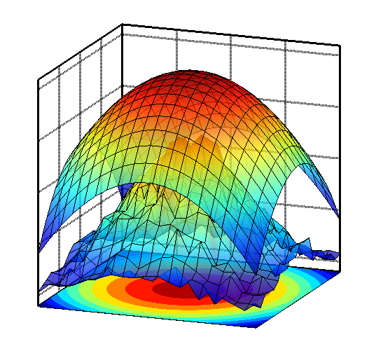
DataMelt (DMelt) is a software for numeric computation, statistics, symbolic calculations, data analysis and data visualization. This multiplatform program combines the simplicity of scripting languages, such as Python, Ruby, Grovy and others with the power of tens of thousands Java classes for numeric computation and visualization.
Welcome to DataMelt
Description
- DataMelt, or DMelt, is software for numeric computation, statistics, analysis of large data volumes ("big data") and scientific visualization. The program can be used in many areas, such as natural sciences, engineering, modeling and analysis of financial markets.
- DMelt is a computational platform. It can be used with different programming languages on different operating systems. Unlike other statistical programs, it is not limited to a single programming language.
- DMelt runs on the Java platform but can be used with the Python language too. Thus this software combines the world's most-popular enterprise language with the most popular scripting language used in data science.
- DataMelt allows the usage of dynamically-typed languages which are significantly faster than the standard Python implemented in C. For example, DataMelt provides Groovy scripting which is a factor 10 faster than Python.
- Python, Groovy, JRuby and Java programming can use more than 50,000 Java classes for numeric computation and scientific visualization. In addition, more than 4000 classes come with Java API, plus 500 native Python modules. Not to mention modules of Groovy and Ruby.
- More than 700 examples for numeric computation and visualization.
- DMelt creates high-quality vector-graphics images (SVG, EPS, PDF etc.) that can be included in LaTeX and other text-processing systems.
Supported programming languages

DataMelt can be used with several scripting languages for the Java platform: Jython (Python programming language), Groovy, JRuby (Ruby programming language) and BeanShell. All scripting languages use common DataMelt JAVA API. Data analyses and statistical computations can be done in JAVA. Finally, symbolic calculations can be done using Matlab/Octave high-level interpreted language integrated with JAVA. Comparisons of performances of these languages are given here.
Supported platforms
DataMelt runs on Windows, Linux, Mac and Android operating systems. The Android application is called AWork. Thus the software represents the ultimate analysis framework which can be used on any hardware, such as desktops, laptops, netbooks, production servers and android tablets. DataMelt is also available on Amazon EC2 cloud.
Portable and commercial friendly
DataMelt is a portable application. No installation is needed: simply download and unzip the package, and you are ready to run it. One can run it from a hard drive, from a USB flash drive or from any media. DataMelt exists as an open-source portable application, and as Java libraries under a commercial friendly license.